Shapes#

A signal is an array of numbers computed once at load time. qps: signal('name', peak: N) points a stage’s rate limiter at one, so the load curve is anything you can write as an expression rather than a constant or a linear ramp(). The same buffer can be read from an arg expression, so the rows carry the value that set their rate.

This page is a catalogue of shapes. It starts with the ten edg ships ready to use, which need no expression at all, then writes shapes from scratch: the expression that declares each one, how several of them run at once, and what they measure like after a real run.

Bundled shapes#

Ten shapes ship with edg. They need no declaration and no expression; just provide the name of the shape you want and give it a peak:

stages {
  soak(workers: 16, duration: 10m, qps: signal('edg-ramp-hold', peak: 2000))
}

Every bundled shape is named with an edg- prefix. Identifiers in a config cannot contain a hyphen, so a shape you declare yourself can never collide with one of these.

The shapes#

Shape	What it does	Reach for it when
`edg-ramp`	Climbs steadily from nothing to full load.	Finding where latency starts to bend.
`edg-staircase`	Climbs in five flat steps, holding each one.	Same question as `edg-ramp`, but each step holds long enough to read a stable p99 off it.
`edg-ramp-hold`	Climbs for a tenth of the run, holds flat, winds back down.	The standard soak: warm the pool, hold, drain.
`edg-business-hours`	One broad rise and fall, quiet at both ends, never idle.	A daily cycle, including what the database gets up to in the trough.
`edg-two-peaks`	A smaller morning rush and a larger evening one.	Consumer traffic, which peaks twice rather than once.
`edg-week`	Seven days of business hours, weekend at a third.	Week-scale work: backup windows, Monday morning against a cold cache.
`edg-spike`	Flat and low, one short burst of five times the load, flat again.	A marketing send or a cache expiry - can the system absorb a burst.
`edg-batch`	Twelve square bursts with near-idle gaps.	Cron and ETL windows, where load arrives with hard edges and no warmup.
`edg-backlog`	Builds up twelve times over, each time dropping to nothing.	Queue consumers and change feeds catching up.
`edg-outage`	Steady, then almost nothing, then a catch-up surge that settles.	Recovery: retry storms and cold caches after something was down.

List them from the terminal with edg signals, or search by name or description with edg signals outage.

What each one looks like#

Each shape below is the expression edg signals --show prints at the shape’s own length, followed by a ten-minute run of it in the TUI. The jitter is real throughput, not the curve.

`edg-ramp`#

i / 288.0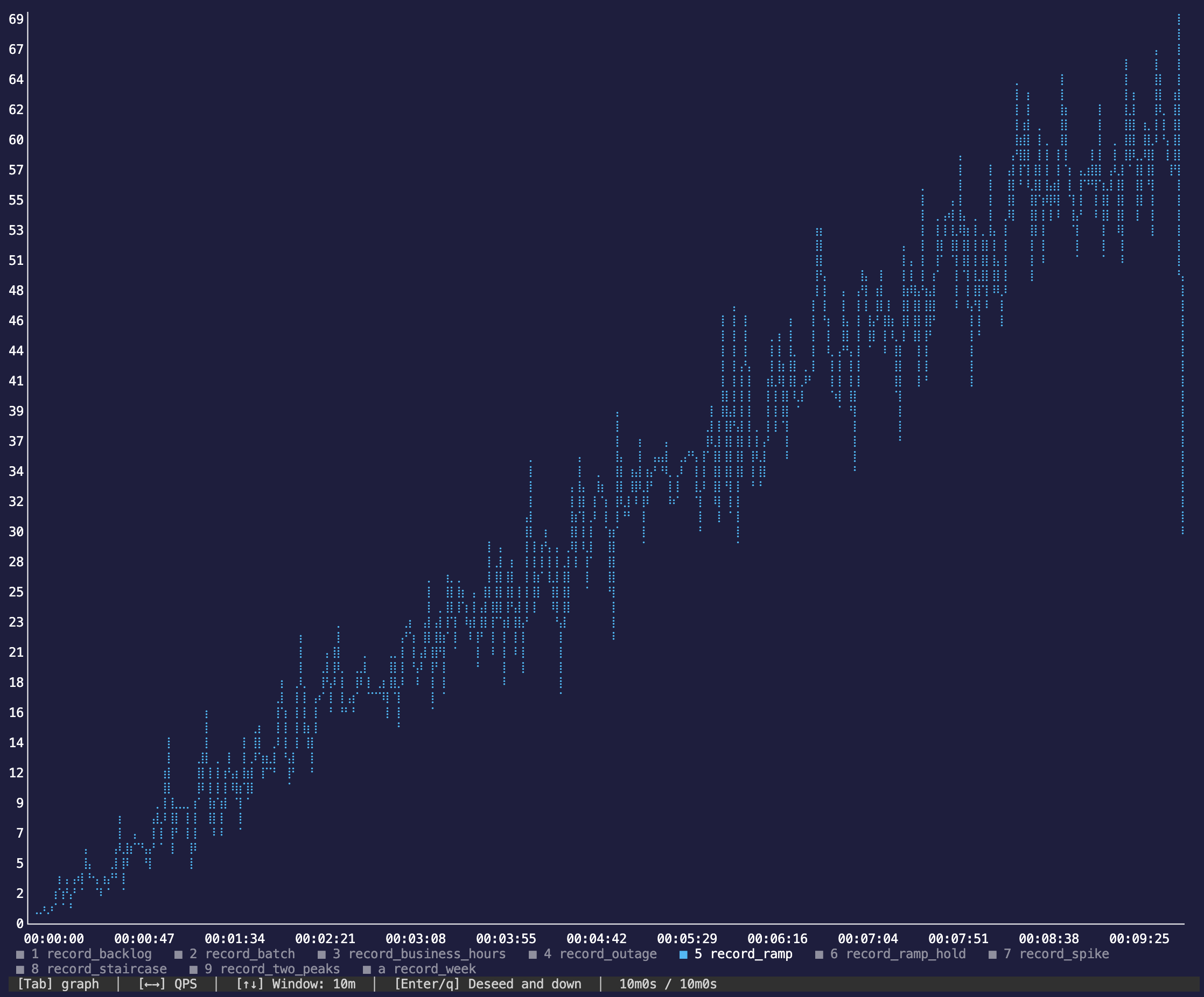

edg-ramp

`edg-staircase`#

(floor(i * 5 / 288.0) + 1) / 5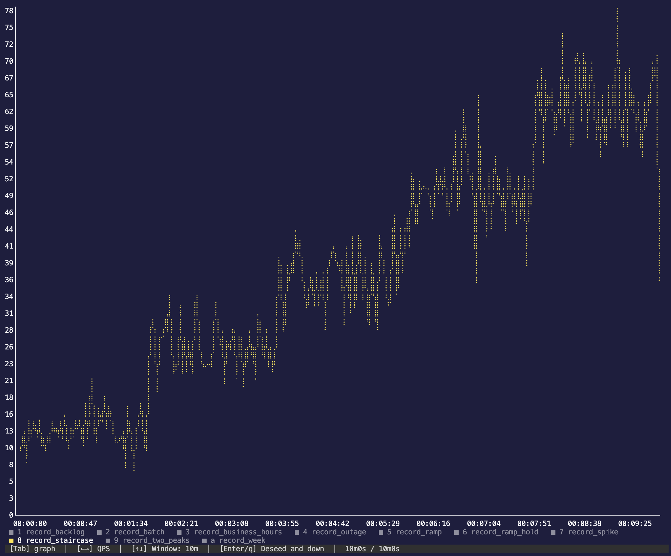

edg-staircase

`edg-ramp-hold`#

cond(i < 28, i / 28.0, cond(i < 260, 1.0, (288 - i) / 28.0))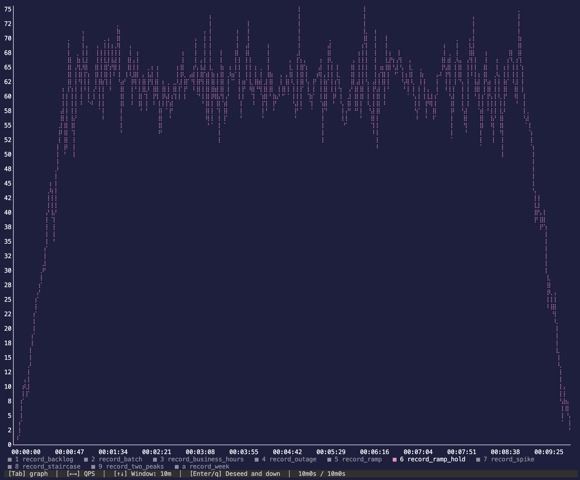

edg-ramp-hold

`edg-business-hours`#

0.15 + 0.85 * pow(sin(pi * i / 288.0), 2)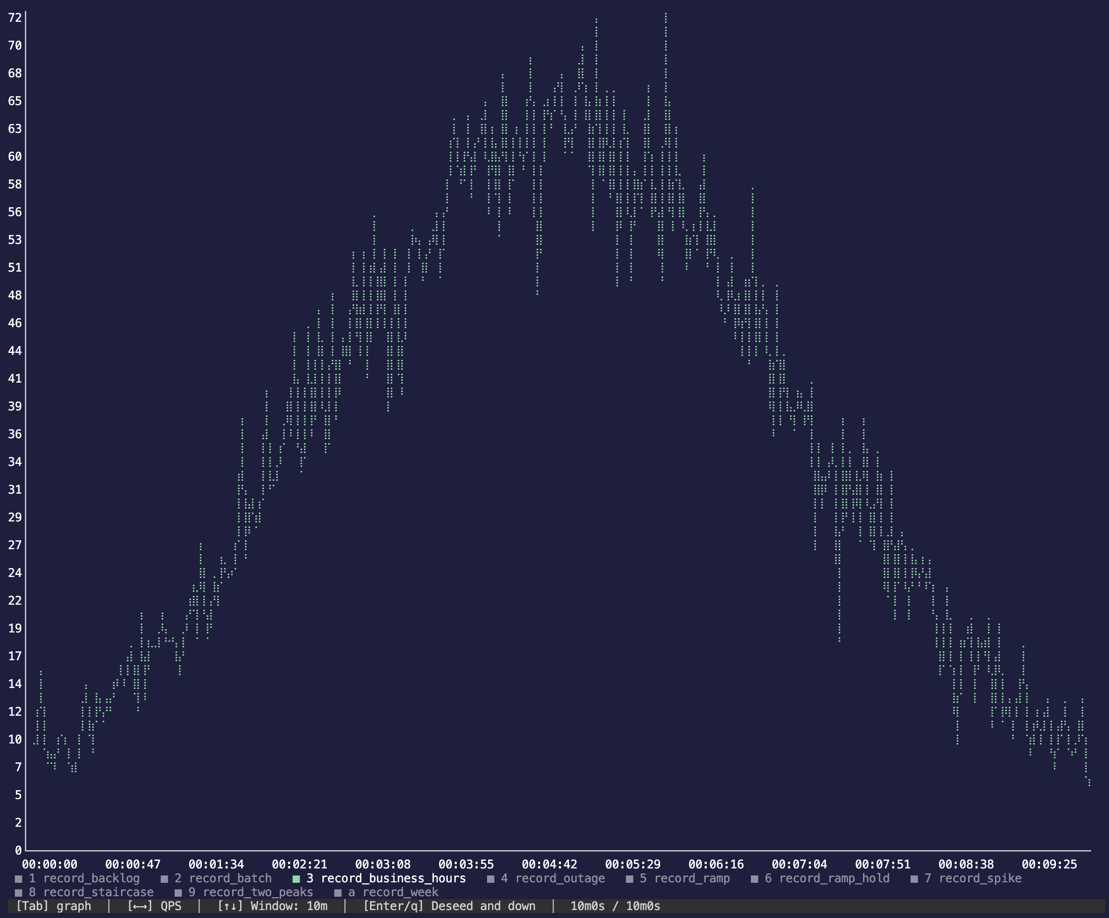

edg-business-hours

`edg-two-peaks`#

0.1 + 0.5 * pow(cos(pi * (i / 288.0 - 0.375)), 24) + 0.9 * pow(cos(pi * (i / 288.0 - 0.833)), 24)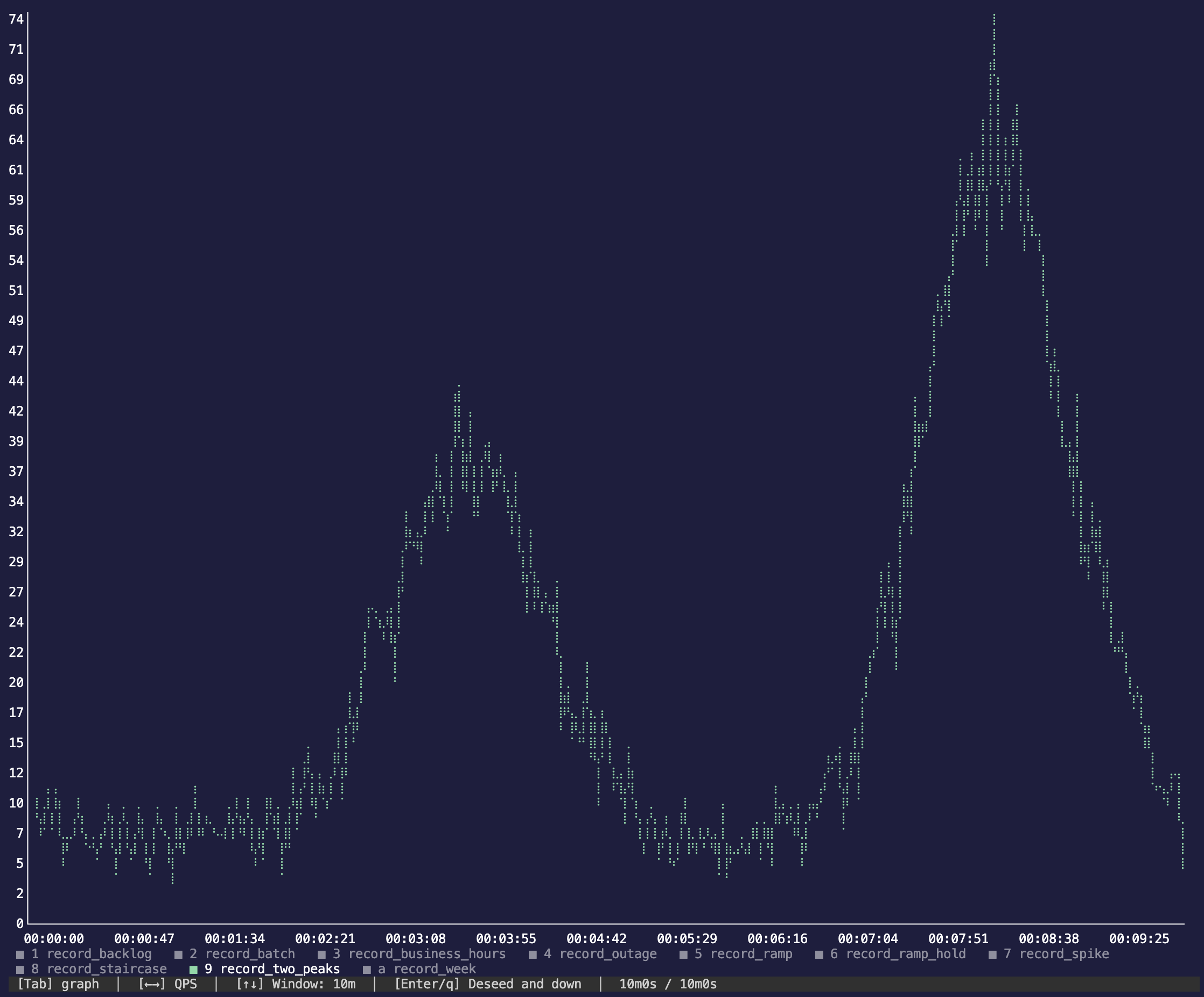

edg-two-peaks

`edg-week`#

cond(floor(i * 7 / 2016.0) < 5, 1.0, 0.35) * (0.15 + 0.85 * pow(sin(pi * mod(i * 7 / 2016.0, 1)), 2))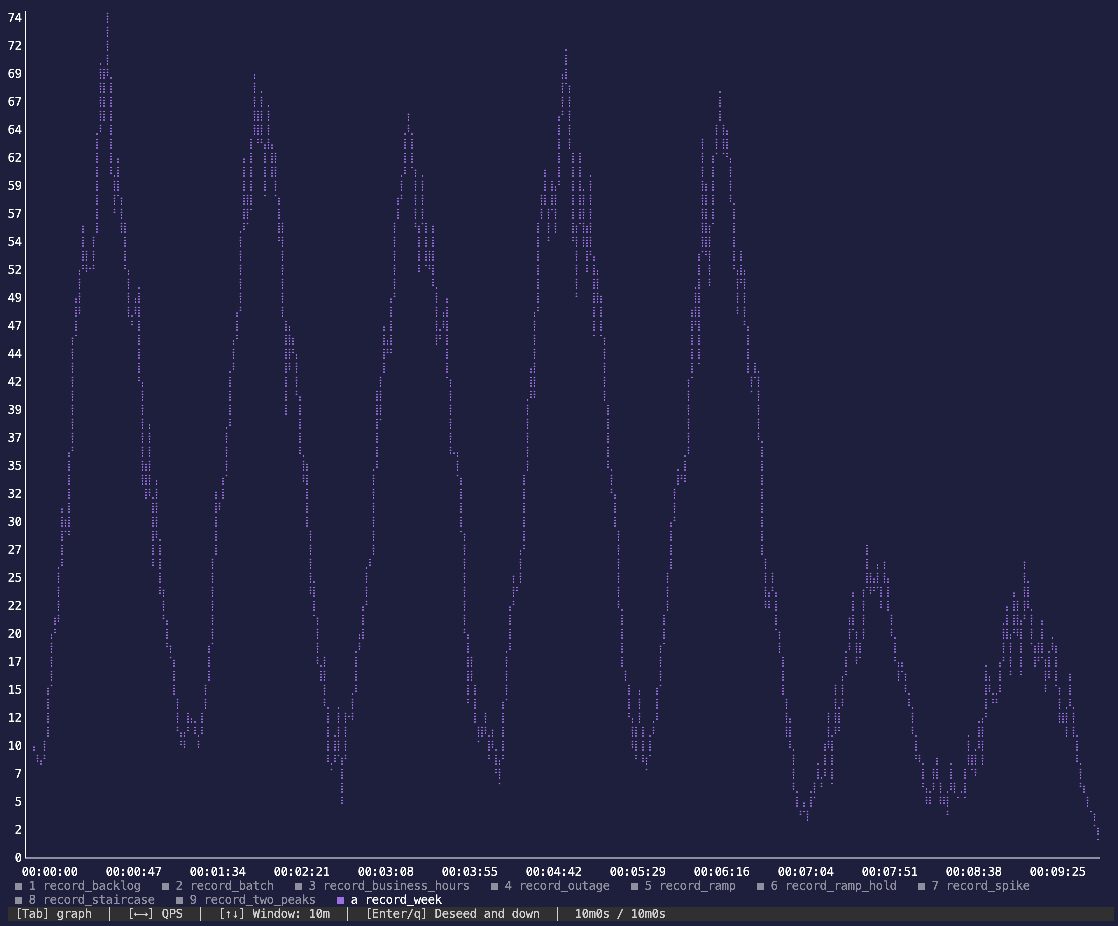

edg-week

`edg-spike`#

0.2 + 0.8 * pow(cos(pi * (i / 288.0 - 0.6)), 200)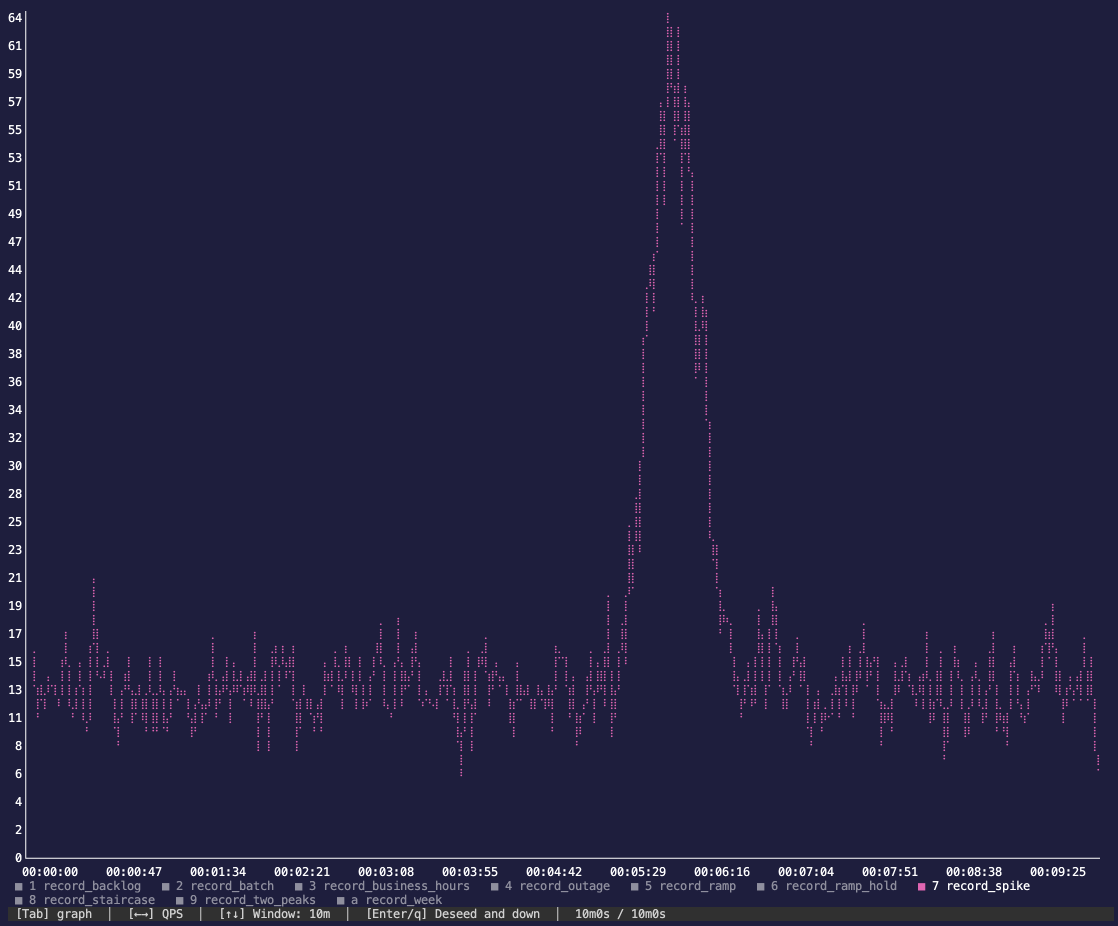

edg-spike

`edg-batch`#

cond(mod(i, 24) < 4, 1.0, 0.1)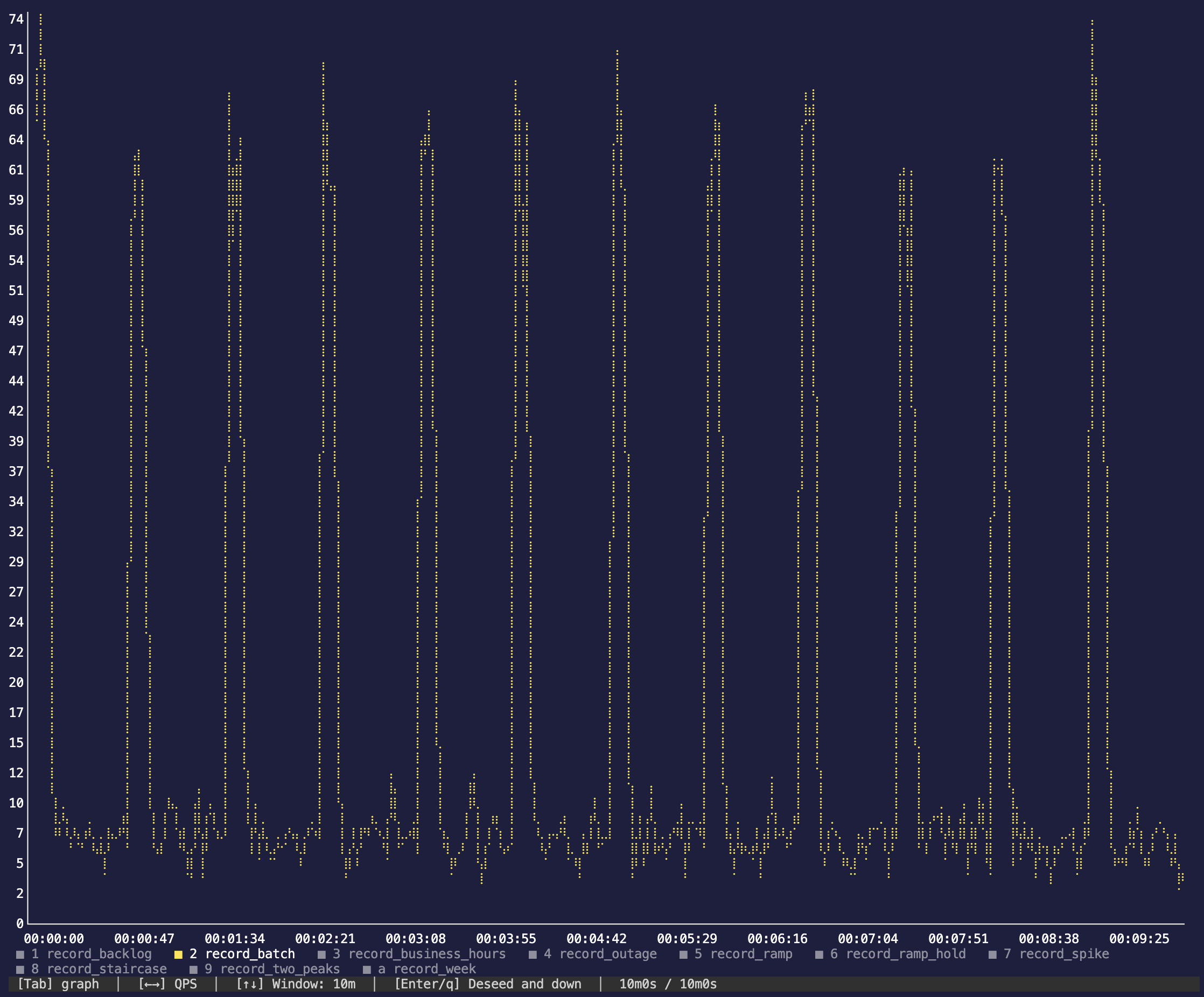

edg-batch

`edg-backlog`#

mod(i, 24) / 24.0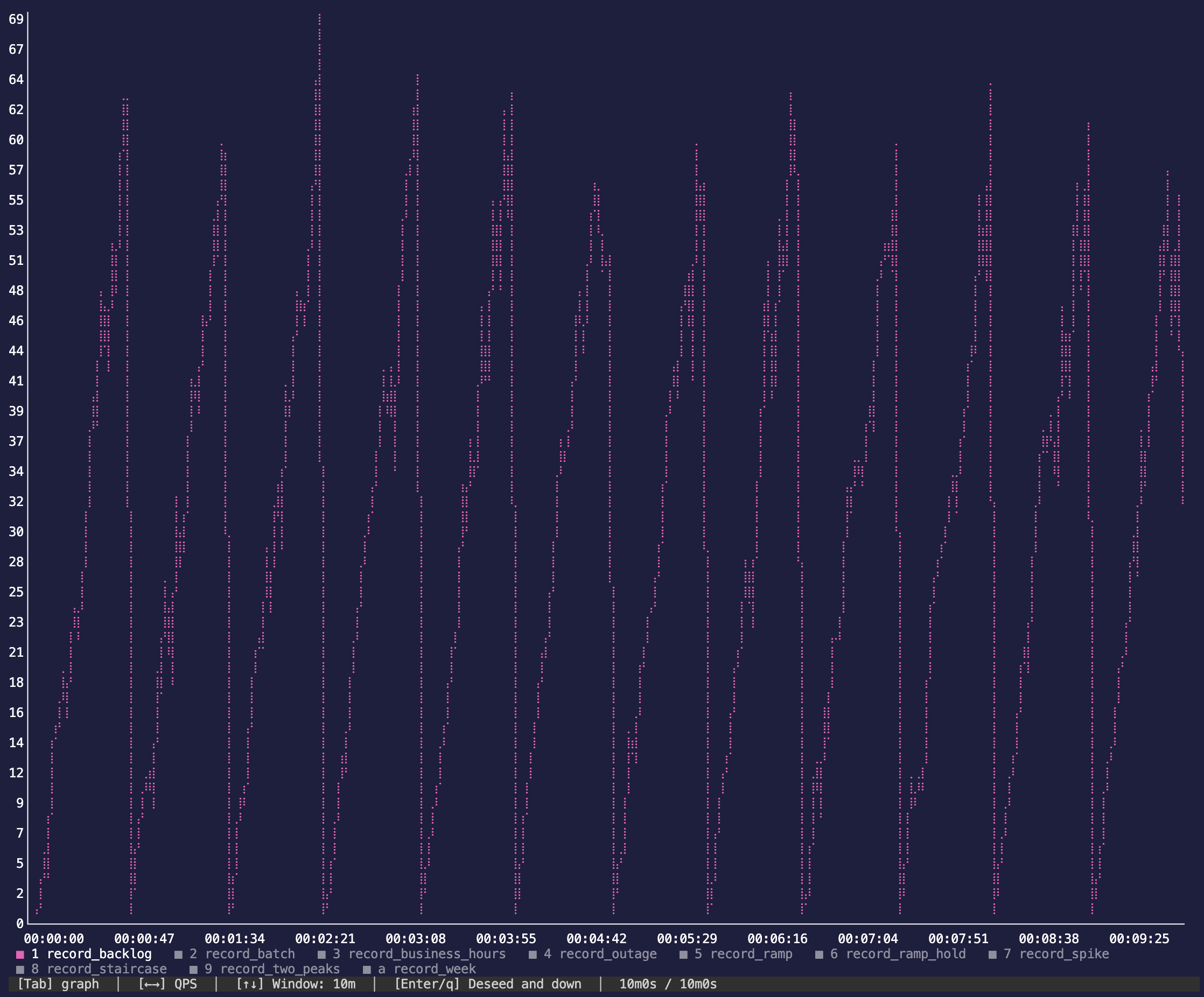

edg-backlog

`edg-outage`#

cond(i < 115, 0.5, cond(i < 144, 0.01, cond(i < 172, 1.0 - 0.5 * (i - 144) / 28.0, 0.5)))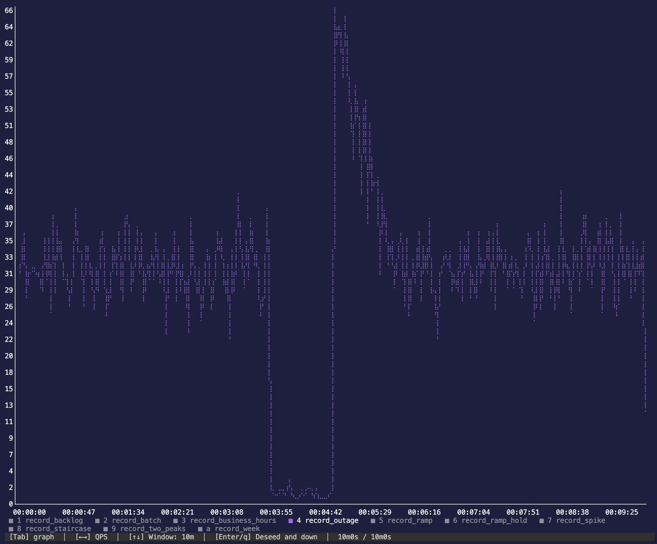

edg-outage

Where `peak` lands#

peak maps the tallest point of a shape to the queries per second you give it and scales the rest proportionally, so the shapes are all written to run between 0 and 1 and peak makes them real. That means peak is not always the load you will see most of the time:

Shape	`peak` lands on	Typical load
`edg-spike`	The top of the burst.	A fifth of `peak` outside it.
`edg-outage`	The top of the catch-up surge.	Half of `peak` either side of it.
`edg-batch`	The rate inside a burst.	A tenth of `peak` in the gaps.
Everything else	The shape’s own high point.	Varies across the curve.

edg signals prints the same note under each shape.

Length (and why 288)#

Nine of the ten shapes declare length: 288, and edg-week declares 7 x 288 = 2016. This number isn’t a duration, it’s a point count. A bundled shape declares a length but no interval, so its length is resolution: the curve is stretched across the whole run, however long that is. A ten-minute run and a ten-hour run both see all 288 points and the full shape. Nothing about 288 pins a bundled shape to a day of wall clock.

288 is a day at five-minute resolution. 24h / 5m = 288. That’s the grid the hand-written shapes further down this page use, and picking the same one means i reads the same way in both: 12 points to the hour, so i / 12.0 is the hour of day. A bundled shape and one you write compose without rescaling.

288 divides cleanly. 288 = 2⁵ x 3², so the constants each shape derives from its length land on whole indices:

Shape	Derived from length `n`	At `n = 288`
`edg-batch`, `edg-backlog`	`n / 12` burst period	24 - two simulated hours per burst
`edg-batch`	`period / 6` burst width	4
`edg-ramp-hold`	`n / 10` ramp	28, holding to 260, with a 28-point descent
`edg-outage`	`n * 4/10`, `n / 2`, `n * 6/10`	115, 144, 172

288 is a default, not a constant. Every shape builds its expression from whatever length it is given, so --length re-derives all of the above: edg signals --show edg-batch --length 1440 has a period of 120, not 24. The only thing the shapes guard against is a length too small to divide, which 288 never is.

Position is measured from the start of the run rather than the start of the stage, so consecutive stages carve up one curve instead of each replaying it from the beginning. A stage that wants a whole shape to itself should be the only stage in the config.

Changing one#

The shapes take no options. To change one, print it as a declaration and edit that:

edg signals --show edg-staircase

# Climbs in five flat steps, holding each one long enough to measure.
signal staircase(length: 288) {
  (floor(i * 5 / 288.0) + 1) / 5
}

Paste it into a config and the 5s become however many steps you want. --length prints the same shape at a different resolution, which matters when you want finer steps or a longer buffer:

edg signals --show edg-business-hours --length 1440

The printed block is the definition the bundled shape itself uses, so a pasted copy behaves identically until you change it. It’s also the quickest way into writing shapes from scratch. The rest of this page covers what the expressions are doing.

To edit one and see what the edit did, edg signal explore opens the same expression in a chart that redraws as you type:

edg signal explore edg-staircase

Anchoring shapes to the clock#

A bundled shape knows where it is in the run, not what time it is. To tie a curve to real timestamps - so a window really does start at 01:00 - print it, then swap length for from, to and interval:

sim(period: '24h', in: '6m', from: '2024-06-03T00:00:00Z')

signal business_hours(from: '2024-06-03T00:00:00Z', to: '2024-06-04T00:00:00Z', interval: '5m') {
  0.15 + 0.85 * pow(sin(pi * i / 288.0), 2)
}

A day at 5m is 288 points, so the expression needs no rescaling - the same grid, now with an interval attached. With a sim block the buffer advances one step per interval of simulated time, so the curve and sim_time() agree on what hour it is.

Combining them#

A signal expression can read any other signal, bundled ones included, so shapes compose into a total the way hand-written ones do:

signal total(length: 288) {
  signal_at('edg-business-hours', i) + 0.5 * signal_at('edg-batch', i)
}

stages {
  day(workers: 16, duration: 10m, qps: signal('total', peak: 1000))
}

Note that peak then normalises against the total, so each shape’s own share is peak x shape / max(total). Running shapes concurrently covers splitting one limiter across several shapes with per-shape queries.

Reading one from an argument#

The same buffer can be read from an argument expression, so rows can carry the value that set their rate:

run {
  record(type: exec) `INSERT INTO events (ts, load) VALUES (now(), $1)` (
    signal('edg-business-hours')
  )
}

One thing to know: signal('name') indexes by the worker’s iteration count, while the stage’s rate limiter indexes by position in the run. The two only line up when iterations happen to tick at the buffer’s pace, so treat the recorded value as the shape rather than as the instantaneous rate. signal_at('name', i) with an index you control avoids the question entirely.

The day#

The rest of this page writes shapes from scratch. Every shape below is 288 points on a 5m interval - the same grid the bundled shapes use, one simulated day - so i / 12.0 is the hour of day. The sim block compresses that day into six minutes of wall clock and anchors the simulated clock to the same instant the signals use, so the curves and sim_time() agree on what hour it is.

A database that serves a business running around the clock does not see one shape at a time. It sees the nightly batch and the hourly crons and the office hump and the background integrations, all at once. Every shape here is live for the whole day; the ones with windows are zero outside them.

sim(period: '24h', in: '6m', from: '2024-06-03T00:00:00Z')

# Background integrations, health checks and monitoring. Flat, always on,
# and the reason the database is never idle.
signal steady(from: '2024-06-03T00:00:00Z', to: '2024-06-04T00:00:00Z', interval: '5m') {
  0.3
}

# A square window. The nightly ETL runs flat out from 01:00 to 03:00 and
# not at all outside it.
signal etl(from: '2024-06-03T00:00:00Z', to: '2024-06-04T00:00:00Z', interval: '5m') {
  cond ( i / 12.0 >= 1 && i / 12.0 < 3 , 1 , 0 )
}

# Office hours. A 5% floor with a sine hump from 08:00 to 18:00 peaking
# at 13:00.
signal workday(from: '2024-06-03T00:00:00Z', to: '2024-06-04T00:00:00Z', interval: '5m') {
  cond ( i / 12.0 >= 8 && i / 12.0 < 18 , 0.05 + 0.95 * pow ( sin ( pi * ( i / 12.0 - 8 ) / 10 ) , 2 ) , 0.05 )
}

# Sharp bursts on the hour, every hour. mod(i, 12) is the position within
# a simulated hour and cos^8 turns that into a narrow spike sitting on an
# 8% baseline.
signal spikes(from: '2024-06-03T00:00:00Z', to: '2024-06-04T00:00:00Z', interval: '5m') {
  0.08 + 0.92 * pow ( cos ( pi * mod ( i , 12 ) / 12 ) , 8 )
}

# A deterministic shape carrying random noise. A broad hump across the
# waking day multiplied by a jitter factor drawn from an empirical CDF of
# four observed values, so the curve is recognisable but no two points
# sit exactly on it.
signal jitter(from: '2024-06-03T00:00:00Z', to: '2024-06-04T00:00:00Z', interval: '5m') {
  ( 0.2 + 0.6 * pow ( sin ( pi * i / 288 ) , 2 ) ) * empirical.float ( [ 0.8 , 1.0 , 1.0 , 1.25 ] , 3 )
}

# A quadratic wind-down across the last two hours of the day.
signal decay(from: '2024-06-03T00:00:00Z', to: '2024-06-04T00:00:00Z', interval: '5m') {
  cond ( i / 12.0 >= 22 , pow ( ( 24 - i / 12.0 ) / 2 , 2 ) , 0 )
}

Shape	Live	Built from
`steady`	all day	A constant. The contrast case.
`etl`	01:00-03:00	`cond()` - hard edges, nothing outside the window.
`workday`	08:00-18:00	`sin^2` hump on a 5% floor.
`spikes`	all day	`cos^8` of the position within the hour, on an 8% baseline.
`jitter`	all day	`sin^2` hump multiplied by an `empirical.float()` draw.
`decay`	22:00-24:00	Quadratic run-down to zero at midnight.

Three rules govern all of them:

peak normalises the buffer, mapping its maximum to the declared QPS and scaling everything else proportionally. A shape written in 0..1 and the same shape written in row counts behave identically, so the expressions above only have to get the shape right.
Position is measured from the start of the run, not the start of the stage, so consecutive stages carve up one timeline instead of each replaying its curve from index 0.
A shape’s maximum must fall inside the stage that uses it. Normalisation is against the whole buffer, so a signal whose tallest point sits outside its stage never reaches the peak it asked for.

Running shapes concurrently#

Stages run one after another, and a stage has one qps, so concurrent shapes cannot come from a stage each. They come from two declarations instead.

First, a composite. A signal expression can read the signals declared above it, so the total the database actually sees is a signal like any other:

signal total(from: '2024-06-03T00:00:00Z', to: '2024-06-04T00:00:00Z', interval: '5m') {
  signal_at ( 'steady' , i ) + signal_at ( 'etl' , i ) + signal_at ( 'workday' , i ) + signal_at ( 'spikes' , i ) + signal_at ( 'jitter' , i ) + signal_at ( 'decay' , i )
}

stages {
  day(workers: 16, duration: 24h, qps: signal('total', peak: 1000))
}

Second, a split. run_weights are static integers, so they cannot follow a curve - but a standalone conditional can. Each run item fires with its own shape’s share of the current instant’s total:

expr share = signal_at(args[0], int(sim_progress() * 288)) / signal_at('total', int(sim_progress() * 288))
expr load  = signal_at(args[0], int(sim_progress() * 288))

run {
  if uniform.float(0.0, 1.0, 6) < share('workday') {
    record_workday(type: exec)
      `INSERT INTO events (ts, shape, load) VALUES ($1, 'workday', $2)` (
        sim_time(),
        load('workday')
      )
  }

  # ...one per shape
}

The shares sum to 1, so an iteration writes one row on average and the limiter’s rate is the row rate. A shape’s expected rate is peak x share, which is peak x shape / total - the shape itself, scaled. Every shape gets its own curve out of one limiter.

Two consequences worth knowing:

No run_weights. Standalone if blocks and run_weights are mutually exclusive, which is fine here: the conditionals are the weights, recomputed every iteration.
peak belongs to the composite. Each shape’s own peak is peak x max(shape) / max(total), so raising one shape lowers every other shape’s share unless peak goes up with it.

Noise as a shape#

jitter is the only shape above that is not purely deterministic. Random generators are available inside signal expressions, but they are evaluated once per index while the buffer is built, so the result is a fixed rough-edged curve rather than live randomness - the same jitter replays every time the buffer wraps.

A generator on its own has no shape at all: draws are independent per index, so a signal of nothing but empirical.float() is frozen white noise with the marginal distribution of the samples. Multiplying a deterministic curve by a jitter factor centred on 1.0 keeps the shape and roughens it. Note that peak then normalises against the tallest draw, and in a composite the draw also moves every other shape’s share, so the exact split changes a little from run to run.

What the shapes measure like#

One six-minute run of the config above, 16 workers against a three-node CockroachDB cluster:

summary
Duration:  6m0.004s
Workers:   16

QUERY           COUNT  ERRORS  p90      p95      p99      QPS
record_decay    3480   0       1.238ms  1.407ms  2.27ms   9.7
record_etl      9810   0       1.332ms  1.566ms  2.672ms  27.2
record_jitter   59779  0       1.273ms  1.4ms    2.083ms  166.1
record_spikes   38983  0       1.24ms   1.369ms  2.193ms  108.3
record_steady   35872  0       1.335ms  1.504ms  2.409ms  99.6
record_workday  29406  0       1.205ms  1.315ms  2.182ms  81.7

Transactions:  177330
Errors:        0
tpm:           29554.7

The QPS column averages over the whole run, so a shape that is only live for two simulated hours reads low. The histograms are where the shapes show up.

The data spans a full simulated day:

SELECT
  min(ts),
  max(ts),
  max(ts) - min(ts) AS span,
  COUNT(*)
FROM events;

              min              |             max              |      span      | count
-------------------------------+------------------------------+----------------+---------
  2024-06-03 00:00:01.90375+00 | 2024-06-03 23:59:59.08748+00 | 23:59:57.18373 | 177330

Every shape starts in the first second of the day except the two with windows, which appear only inside theirs:

SELECT
  shape,
  min(ts)::TIME AS from_t,
  max(ts)::TIME AS to_t,
  COUNT(*) AS n
FROM events
GROUP BY shape
ORDER BY min(ts);

   shape  |     from_t     |      to_t      |   n
----------+----------------+----------------+--------
  spikes  | 00:00:01.90375 | 23:59:59.08748 | 38983
  jitter  | 00:00:03.58447 | 23:59:58.04464 | 59779
  workday | 00:00:04.01565 | 23:59:57.56771 | 29406
  steady  | 00:00:04.94541 | 23:59:54.90739 | 35872
  etl     | 01:00:00.14997 | 02:59:58.85711 |  9810
  decay   | 22:00:00.27498 | 23:54:29.6773  |  3480

etl lands on its window to within a fraction of a simulated second at both ends, without the stage and the signal having to agree on a boundary twice.

The whole day, hour by hour#

SELECT
  extract(hour FROM ts)::INT AS hour,
  COUNT(*) AS n,
  repeat('▒', (COUNT(*)::FLOAT8 / max(COUNT(*)) OVER () * 40)::INT) AS bar
FROM events
GROUP BY hour
ORDER BY hour;

  hour |   n   |                   bar
-------+-------+-------------------------------------------
     0 |  4546 | ▒▒▒▒▒▒▒▒▒▒▒▒▒▒▒
     1 |  9457 | ▒▒▒▒▒▒▒▒▒▒▒▒▒▒▒▒▒▒▒▒▒▒▒▒▒▒▒▒▒▒▒▒
     2 |  9495 | ▒▒▒▒▒▒▒▒▒▒▒▒▒▒▒▒▒▒▒▒▒▒▒▒▒▒▒▒▒▒▒▒
     3 |  4801 | ▒▒▒▒▒▒▒▒▒▒▒▒▒▒▒▒
     4 |  5382 | ▒▒▒▒▒▒▒▒▒▒▒▒▒▒▒▒▒▒
     5 |  5569 | ▒▒▒▒▒▒▒▒▒▒▒▒▒▒▒▒▒▒▒
     6 |  6071 | ▒▒▒▒▒▒▒▒▒▒▒▒▒▒▒▒▒▒▒▒▒
     7 |  6532 | ▒▒▒▒▒▒▒▒▒▒▒▒▒▒▒▒▒▒▒▒▒▒
     8 |  6902 | ▒▒▒▒▒▒▒▒▒▒▒▒▒▒▒▒▒▒▒▒▒▒▒
     9 |  7977 | ▒▒▒▒▒▒▒▒▒▒▒▒▒▒▒▒▒▒▒▒▒▒▒▒▒▒▒
    10 |  9644 | ▒▒▒▒▒▒▒▒▒▒▒▒▒▒▒▒▒▒▒▒▒▒▒▒▒▒▒▒▒▒▒▒▒
    11 | 10780 | ▒▒▒▒▒▒▒▒▒▒▒▒▒▒▒▒▒▒▒▒▒▒▒▒▒▒▒▒▒▒▒▒▒▒▒▒▒
    12 | 11758 | ▒▒▒▒▒▒▒▒▒▒▒▒▒▒▒▒▒▒▒▒▒▒▒▒▒▒▒▒▒▒▒▒▒▒▒▒▒▒▒▒
    13 | 11633 | ▒▒▒▒▒▒▒▒▒▒▒▒▒▒▒▒▒▒▒▒▒▒▒▒▒▒▒▒▒▒▒▒▒▒▒▒▒▒▒▒
    14 | 10858 | ▒▒▒▒▒▒▒▒▒▒▒▒▒▒▒▒▒▒▒▒▒▒▒▒▒▒▒▒▒▒▒▒▒▒▒▒▒
    15 |  9186 | ▒▒▒▒▒▒▒▒▒▒▒▒▒▒▒▒▒▒▒▒▒▒▒▒▒▒▒▒▒▒▒
    16 |  7434 | ▒▒▒▒▒▒▒▒▒▒▒▒▒▒▒▒▒▒▒▒▒▒▒▒▒
    17 |  6436 | ▒▒▒▒▒▒▒▒▒▒▒▒▒▒▒▒▒▒▒▒▒▒
    18 |  5712 | ▒▒▒▒▒▒▒▒▒▒▒▒▒▒▒▒▒▒▒
    19 |  5180 | ▒▒▒▒▒▒▒▒▒▒▒▒▒▒▒▒▒▒
    20 |  4879 | ▒▒▒▒▒▒▒▒▒▒▒▒▒▒▒▒▒
    21 |  4716 | ▒▒▒▒▒▒▒▒▒▒▒▒▒▒▒▒
    22 |  7468 | ▒▒▒▒▒▒▒▒▒▒▒▒▒▒▒▒▒▒▒▒▒▒▒▒▒
    23 |  4914 | ▒▒▒▒▒▒▒▒▒▒▒▒▒▒▒▒▒

This is the composite, and it reads like a working day: a batch window overnight, a long climb to a midday peak, a decline through the afternoon, and a bump at 22:00 as the wind-down starts.

Split by shape, the same rows show six curves running at once:

SELECT
  extract(hour FROM ts)::INT AS hour,
  COUNT(*) FILTER (WHERE shape = 'steady')  AS steady,
  COUNT(*) FILTER (WHERE shape = 'etl')     AS etl,
  COUNT(*) FILTER (WHERE shape = 'workday') AS workday,
  COUNT(*) FILTER (WHERE shape = 'spikes')  AS spikes,
  COUNT(*) FILTER (WHERE shape = 'jitter')  AS jitter,
  COUNT(*) FILTER (WHERE shape = 'decay')   AS decay
FROM events
GROUP BY hour
ORDER BY hour;

  hour | steady | etl  | workday | spikes | jitter | decay
-------+--------+------+---------+--------+--------+--------
     0 |   1565 |    0 |     263 |   1654 |   1064 |     0
     1 |   1484 | 4955 |     242 |   1624 |   1152 |     0
     2 |   1461 | 4855 |     246 |   1600 |   1333 |     0
     3 |   1416 |    0 |     265 |   1574 |   1546 |     0
     4 |   1556 |    0 |     268 |   1607 |   1951 |     0
     5 |   1522 |    0 |     260 |   1539 |   2248 |     0
     6 |   1535 |    0 |     245 |   1661 |   2630 |     0
     7 |   1494 |    0 |     260 |   1620 |   3158 |     0
     8 |   1507 |    0 |     357 |   1662 |   3376 |     0
     9 |   1460 |    0 |    1194 |   1640 |   3683 |     0
    10 |   1541 |    0 |    2583 |   1702 |   3818 |     0
    11 |   1444 |    0 |    3827 |   1611 |   3898 |     0
    12 |   1443 |    0 |    4736 |   1591 |   3988 |     0
    13 |   1487 |    0 |    4763 |   1603 |   3780 |     0
    14 |   1542 |    0 |    4014 |   1665 |   3637 |     0
    15 |   1513 |    0 |    2676 |   1650 |   3347 |     0
    16 |   1468 |    0 |    1267 |   1567 |   3132 |     0
    17 |   1545 |    0 |     462 |   1657 |   2772 |     0
    18 |   1513 |    0 |     266 |   1614 |   2319 |     0
    19 |   1439 |    0 |     226 |   1617 |   1898 |     0
    20 |   1486 |    0 |     262 |   1631 |   1500 |     0
    21 |   1483 |    0 |     235 |   1648 |   1350 |     0
    22 |   1425 |    0 |     265 |   1608 |   1176 |  2994
    23 |   1543 |    0 |     224 |   1638 |   1023 |   486

steady holds ~1,500 rows an hour from midnight to midnight and spikes ~1,620 (its bursts average flat at this resolution), while workday climbs 20x into its hump, jitter traces a broad rise and fall, and etl and decay occupy their windows. Nothing here is a stage boundary; every column is competing for the same limiter the whole time.

The square window#

The etl shape, in half-hour buckets. It is square because the cond() that declares it has no ramp at either end: the signal is 1 inside 01:00-03:00 and 0 outside, so load goes from idle to full share between two adjacent buffer points and back again.

SELECT
  to_char(date_trunc('hour', ts) + INTERVAL '30 minutes' * floor(extract(minute FROM ts) / 30), 'HH24:MI') AS bucket,
  COUNT(*) AS n,
  repeat('▒', (COUNT(*)::FLOAT8 / max(COUNT(*)) OVER () * 40)::INT) AS bar
FROM events
WHERE shape = 'etl'
GROUP BY bucket
ORDER BY bucket;

  bucket |  n   |                   bar
---------+------+-------------------------------------------
  01:00  | 2435 | ▒▒▒▒▒▒▒▒▒▒▒▒▒▒▒▒▒▒▒▒▒▒▒▒▒▒▒▒▒▒▒▒▒▒▒▒▒▒▒
  01:30  | 2520 | ▒▒▒▒▒▒▒▒▒▒▒▒▒▒▒▒▒▒▒▒▒▒▒▒▒▒▒▒▒▒▒▒▒▒▒▒▒▒▒▒
  02:00  | 2467 | ▒▒▒▒▒▒▒▒▒▒▒▒▒▒▒▒▒▒▒▒▒▒▒▒▒▒▒▒▒▒▒▒▒▒▒▒▒▒▒
  02:30  | 2388 | ▒▒▒▒▒▒▒▒▒▒▒▒▒▒▒▒▒▒▒▒▒▒▒▒▒▒▒▒▒▒▒▒▒▒▒▒▒▒

Four buckets, nothing either side, and the four within 5% of each other. The edges are as sharp as the cond() that declared them.

The hourly bursts#

spikes is live all day, so the hourly bucket flattens it. Drop to ten minutes over any two hours and the bursts appear:

SELECT
  to_char(date_trunc('hour', ts) + INTERVAL '10 minutes' * floor(extract(minute FROM ts) / 10), 'HH24:MI') AS bucket,
  COUNT(*) AS n,
  repeat('▒', (COUNT(*)::FLOAT8 / max(COUNT(*)) OVER () * 40)::INT) AS bar
FROM events
WHERE shape = 'spikes'
  AND ts >= '2024-06-03 12:00:00' AND ts < '2024-06-03 14:00:00'
GROUP BY bucket
ORDER BY bucket;

  bucket |  n  |                   bar
---------+-----+-------------------------------------------
  12:00  | 708 | ▒▒▒▒▒▒▒▒▒▒▒▒▒▒▒▒▒▒▒▒▒▒▒▒▒▒▒▒▒▒▒▒▒▒▒▒▒▒▒▒
  12:10  | 197 | ▒▒▒▒▒▒▒▒▒▒▒
  12:20  |  59 | ▒▒▒
  12:30  |  63 | ▒▒▒▒
  12:40  |  77 | ▒▒▒▒
  12:50  | 487 | ▒▒▒▒▒▒▒▒▒▒▒▒▒▒▒▒▒▒▒▒▒▒▒▒▒▒▒▒
  13:00  | 707 | ▒▒▒▒▒▒▒▒▒▒▒▒▒▒▒▒▒▒▒▒▒▒▒▒▒▒▒▒▒▒▒▒▒▒▒▒▒▒▒▒
  13:10  | 218 | ▒▒▒▒▒▒▒▒▒▒▒▒
  13:20  |  57 | ▒▒▒
  13:30  |  70 | ▒▒▒▒
  13:40  | 102 | ▒▒▒▒▒▒
  13:50  | 449 | ▒▒▒▒▒▒▒▒▒▒▒▒▒▒▒▒▒▒▒▒▒▒▒▒▒▒▒▒

708 and 707 rows on consecutive hours: cos^8 reproduces itself to within one row a hundred simulated minutes later, in the middle of the busiest part of the day.

The empirical shape#

jitter is a sin^2 hump over the whole day multiplied by an empirical.float([0.8, 1.0, 1.0, 1.25], 3) draw. At day scale, the hump:

SELECT
  extract(hour FROM ts)::INT AS hour,
  COUNT(*) AS n,
  repeat('▒', (COUNT(*)::FLOAT8 / max(COUNT(*)) OVER () * 40)::INT) AS bar
FROM events
WHERE shape = 'jitter'
GROUP BY hour
ORDER BY hour;

  hour |  n   |                   bar
-------+------+-------------------------------------------
     0 | 1064 | ▒▒▒▒▒▒▒▒▒▒▒
     1 | 1152 | ▒▒▒▒▒▒▒▒▒▒▒▒
     2 | 1333 | ▒▒▒▒▒▒▒▒▒▒▒▒▒
     3 | 1546 | ▒▒▒▒▒▒▒▒▒▒▒▒▒▒▒▒
     4 | 1951 | ▒▒▒▒▒▒▒▒▒▒▒▒▒▒▒▒▒▒▒▒
     5 | 2248 | ▒▒▒▒▒▒▒▒▒▒▒▒▒▒▒▒▒▒▒▒▒▒▒
     6 | 2630 | ▒▒▒▒▒▒▒▒▒▒▒▒▒▒▒▒▒▒▒▒▒▒▒▒▒▒
     7 | 3158 | ▒▒▒▒▒▒▒▒▒▒▒▒▒▒▒▒▒▒▒▒▒▒▒▒▒▒▒▒▒▒▒▒
     8 | 3376 | ▒▒▒▒▒▒▒▒▒▒▒▒▒▒▒▒▒▒▒▒▒▒▒▒▒▒▒▒▒▒▒▒▒▒
     9 | 3683 | ▒▒▒▒▒▒▒▒▒▒▒▒▒▒▒▒▒▒▒▒▒▒▒▒▒▒▒▒▒▒▒▒▒▒▒▒▒
    10 | 3818 | ▒▒▒▒▒▒▒▒▒▒▒▒▒▒▒▒▒▒▒▒▒▒▒▒▒▒▒▒▒▒▒▒▒▒▒▒▒▒
    11 | 3898 | ▒▒▒▒▒▒▒▒▒▒▒▒▒▒▒▒▒▒▒▒▒▒▒▒▒▒▒▒▒▒▒▒▒▒▒▒▒▒▒
    12 | 3988 | ▒▒▒▒▒▒▒▒▒▒▒▒▒▒▒▒▒▒▒▒▒▒▒▒▒▒▒▒▒▒▒▒▒▒▒▒▒▒▒▒
    13 | 3780 | ▒▒▒▒▒▒▒▒▒▒▒▒▒▒▒▒▒▒▒▒▒▒▒▒▒▒▒▒▒▒▒▒▒▒▒▒▒▒
    14 | 3637 | ▒▒▒▒▒▒▒▒▒▒▒▒▒▒▒▒▒▒▒▒▒▒▒▒▒▒▒▒▒▒▒▒▒▒▒▒
    15 | 3347 | ▒▒▒▒▒▒▒▒▒▒▒▒▒▒▒▒▒▒▒▒▒▒▒▒▒▒▒▒▒▒▒▒▒▒
    16 | 3132 | ▒▒▒▒▒▒▒▒▒▒▒▒▒▒▒▒▒▒▒▒▒▒▒▒▒▒▒▒▒▒▒
    17 | 2772 | ▒▒▒▒▒▒▒▒▒▒▒▒▒▒▒▒▒▒▒▒▒▒▒▒▒▒▒▒
    18 | 2319 | ▒▒▒▒▒▒▒▒▒▒▒▒▒▒▒▒▒▒▒▒▒▒▒
    19 | 1898 | ▒▒▒▒▒▒▒▒▒▒▒▒▒▒▒▒▒▒▒
    20 | 1500 | ▒▒▒▒▒▒▒▒▒▒▒▒▒▒▒
    21 | 1350 | ▒▒▒▒▒▒▒▒▒▒▒▒▒▒
    22 | 1176 | ▒▒▒▒▒▒▒▒▒▒▒▒
    23 | 1023 | ▒▒▒▒▒▒▒▒▒▒

An hour holds twelve buffer points, so averaging hides the noise. The load column carries the buffer value that set each row’s rate, so reading it back at buffer resolution shows the draw itself:

SELECT
  to_char(date_trunc('hour', ts) + INTERVAL '5 minutes' * floor(extract(minute FROM ts) / 5), 'HH24:MI') AS bucket,
  round(max(load)::NUMERIC, 3) AS load,
  repeat('▒', (max(load)::FLOAT8 / max(max(load)) OVER () * 40)::INT) AS bar
FROM events
WHERE shape = 'jitter'
  AND ts >= '2024-06-03 06:00:00' AND ts < '2024-06-03 08:00:00'
GROUP BY bucket
ORDER BY bucket;

  bucket | load  |                   bar
---------+-------+-------------------------------------------
  06:00  | 0.616 | ▒▒▒▒▒▒▒▒▒▒▒▒▒▒▒▒▒▒▒▒▒▒▒▒▒▒▒▒▒▒▒
  06:05  | 0.629 | ▒▒▒▒▒▒▒▒▒▒▒▒▒▒▒▒▒▒▒▒▒▒▒▒▒▒▒▒▒▒▒
  06:10  | 0.626 | ▒▒▒▒▒▒▒▒▒▒▒▒▒▒▒▒▒▒▒▒▒▒▒▒▒▒▒▒▒▒▒
  06:15  | 0.613 | ▒▒▒▒▒▒▒▒▒▒▒▒▒▒▒▒▒▒▒▒▒▒▒▒▒▒▒▒▒▒▒
  06:20  | 0.641 | ▒▒▒▒▒▒▒▒▒▒▒▒▒▒▒▒▒▒▒▒▒▒▒▒▒▒▒▒▒▒▒▒
  06:25  | 0.655 | ▒▒▒▒▒▒▒▒▒▒▒▒▒▒▒▒▒▒▒▒▒▒▒▒▒▒▒▒▒▒▒▒▒
  06:30  | 0.648 | ▒▒▒▒▒▒▒▒▒▒▒▒▒▒▒▒▒▒▒▒▒▒▒▒▒▒▒▒▒▒▒▒
  06:35  | 0.671 | ▒▒▒▒▒▒▒▒▒▒▒▒▒▒▒▒▒▒▒▒▒▒▒▒▒▒▒▒▒▒▒▒▒
  06:40  | 0.663 | ▒▒▒▒▒▒▒▒▒▒▒▒▒▒▒▒▒▒▒▒▒▒▒▒▒▒▒▒▒▒▒▒▒
  06:45  | 0.695 | ▒▒▒▒▒▒▒▒▒▒▒▒▒▒▒▒▒▒▒▒▒▒▒▒▒▒▒▒▒▒▒▒▒▒▒
  06:50  | 0.694 | ▒▒▒▒▒▒▒▒▒▒▒▒▒▒▒▒▒▒▒▒▒▒▒▒▒▒▒▒▒▒▒▒▒▒▒
  06:55  | 0.689 | ▒▒▒▒▒▒▒▒▒▒▒▒▒▒▒▒▒▒▒▒▒▒▒▒▒▒▒▒▒▒▒▒▒▒
  07:00  | 0.666 | ▒▒▒▒▒▒▒▒▒▒▒▒▒▒▒▒▒▒▒▒▒▒▒▒▒▒▒▒▒▒▒▒▒
  07:05  | 0.703 | ▒▒▒▒▒▒▒▒▒▒▒▒▒▒▒▒▒▒▒▒▒▒▒▒▒▒▒▒▒▒▒▒▒▒▒
  07:10  | 0.655 | ▒▒▒▒▒▒▒▒▒▒▒▒▒▒▒▒▒▒▒▒▒▒▒▒▒▒▒▒▒▒▒▒▒
  07:15  | 0.692 | ▒▒▒▒▒▒▒▒▒▒▒▒▒▒▒▒▒▒▒▒▒▒▒▒▒▒▒▒▒▒▒▒▒▒▒
  07:20  | 0.732 | ▒▒▒▒▒▒▒▒▒▒▒▒▒▒▒▒▒▒▒▒▒▒▒▒▒▒▒▒▒▒▒▒▒▒▒▒
  07:25  | 0.727 | ▒▒▒▒▒▒▒▒▒▒▒▒▒▒▒▒▒▒▒▒▒▒▒▒▒▒▒▒▒▒▒▒▒▒▒▒
  07:30  | 0.653 | ▒▒▒▒▒▒▒▒▒▒▒▒▒▒▒▒▒▒▒▒▒▒▒▒▒▒▒▒▒▒▒▒▒
  07:35  | 0.776 | ▒▒▒▒▒▒▒▒▒▒▒▒▒▒▒▒▒▒▒▒▒▒▒▒▒▒▒▒▒▒▒▒▒▒▒▒▒▒▒
  07:40  | 0.703 | ▒▒▒▒▒▒▒▒▒▒▒▒▒▒▒▒▒▒▒▒▒▒▒▒▒▒▒▒▒▒▒▒▒▒▒
  07:45  | 0.788 | ▒▒▒▒▒▒▒▒▒▒▒▒▒▒▒▒▒▒▒▒▒▒▒▒▒▒▒▒▒▒▒▒▒▒▒▒▒▒▒
  07:50  | 0.796 | ▒▒▒▒▒▒▒▒▒▒▒▒▒▒▒▒▒▒▒▒▒▒▒▒▒▒▒▒▒▒▒▒▒▒▒▒▒▒▒▒
  07:55  | 0.802 | ▒▒▒▒▒▒▒▒▒▒▒▒▒▒▒▒▒▒▒▒▒▒▒▒▒▒▒▒▒▒▒▒▒▒▒▒▒▒▒▒

Rising across the two hours, as the underlying sin^2 says it should, but never monotonically: 07:30 drops to 0.653 between neighbours at 0.727 and 0.776. That dip is a low draw from the CDF, and it is in the buffer for good - the shape is the same every time the run reaches 07:30, which is what makes a noisy curve reproducible rather than merely random.

The wind-down#

SELECT
  to_char(date_trunc('hour', ts) + INTERVAL '15 minutes' * floor(extract(minute FROM ts) / 15), 'HH24:MI') AS bucket,
  COUNT(*) AS n,
  repeat('▒', (COUNT(*)::FLOAT8 / max(COUNT(*)) OVER () * 40)::INT) AS bar
FROM events
WHERE shape = 'decay'
GROUP BY bucket
ORDER BY bucket;

  bucket |  n   |                   bar
---------+------+-------------------------------------------
  22:00  | 1091 | ▒▒▒▒▒▒▒▒▒▒▒▒▒▒▒▒▒▒▒▒▒▒▒▒▒▒▒▒▒▒▒▒▒▒▒▒▒▒▒▒
  22:15  |  840 | ▒▒▒▒▒▒▒▒▒▒▒▒▒▒▒▒▒▒▒▒▒▒▒▒▒▒▒▒▒▒▒
  22:30  |  610 | ▒▒▒▒▒▒▒▒▒▒▒▒▒▒▒▒▒▒▒▒▒▒
  22:45  |  453 | ▒▒▒▒▒▒▒▒▒▒▒▒▒▒▒▒▒
  23:00  |  262 | ▒▒▒▒▒▒▒▒▒▒
  23:15  |  142 | ▒▒▒▒▒
  23:30  |   66 | ▒▒
  23:45  |   16 | ▒

pow((24 - hour) / 2, 2) as a curve of counts: each bucket roughly three quarters of the last.

Peaks against what was declared#

peak: 1000 is the composite’s ceiling, so each shape’s own ceiling is a share of it. The buffer maxima for this config are steady 0.3, jitter ~0.98 (it depends on the draw) and 1.0 for the rest, against a composite maximum of ~3.19 - so the four unit shapes are worth about 314 QPS each at their own peaks and steady about 94.

A 5m simulated bucket is 1.25s of wall clock at 240x, so dividing by that converts rows per bucket into real QPS:

WITH buckets AS (
  SELECT
    shape,
    date_trunc('hour', ts) + INTERVAL '5 minutes' * floor(extract(minute FROM ts) / 5) AS bucket,
    COUNT(*) AS n
  FROM events
  GROUP BY shape, bucket
)
SELECT shape, (max(n) / 1.25)::INT AS peak_qps
FROM buckets
GROUP BY shape
ORDER BY peak_qps DESC;

   shape  | peak_qps
----------+-----------
  etl     |      358
  spikes  |      355
  workday |      355
  decay   |      320
  jitter  |      291
  steady  |      125

The four unit shapes land together, as they should. They read above 314 because max() over 288 buckets picks the luckiest one: each shape’s arrivals are a random draw against its share, so the busiest bucket overstates the rate - most visibly for steady, whose 125 is the tallest of 288 buckets around a true 94. The mean rate over a flat window is the honest check: etl wrote 9,810 rows across two simulated hours, which is 30s of wall clock, for 327 QPS - a few percent above 314 because that run’s own jitter draw set a slightly lower composite maximum, and every other shape’s share rises when it does.

Set workers high enough to sustain the composite peak, exactly as for a flat qps. If the pool saturates, the limiter stops being the binding constraint and every shape flattens together.

Load values travel with the rows#

Each query writes the buffer value that set its rate, so the payload and the arrival pattern come from the same declaration:

SELECT
  shape,
  round(min(load)::NUMERIC, 3) AS min_load,
  round(max(load)::NUMERIC, 3) AS max_load
FROM events
GROUP BY shape
ORDER BY shape;

   shape  | min_load | max_load
----------+----------+-----------
  decay   |    0.007 |    1.000
  etl     |    1.000 |    1.000
  jitter  |    0.161 |    0.999
  spikes  |    0.080 |    1.000
  steady  |    0.300 |    0.300
  workday |    0.050 |    1.000

Every curve’s floor and ceiling, read back out of the table: the 5% workday floor, the 8% spikes baseline, the flat 0.3 of steady, and etl at exactly 1.0 for every row it wrote, because it only writes rows where its square window is up.

Shaping one config per submission#

A shape hard-coded into a signal is one shape. Pull its parameters out through env_nil() and the same file describes a family of them:

let peak_hour = float(coalesce(env_nil('SHAPE_PEAK_HOUR'), 13))
let amp = float(coalesce(env_nil('SHAPE_AMP'), 0.95))
let workers = int(coalesce(env_nil('WORKERS'), 8))

signal workday(from: '2024-06-03T00:00:00Z', to: '2024-06-04T00:00:00Z', interval: '5m') {
  cond ( i / 12.0 >= 8 && i / 12.0 < 18 , 0.05 + amp * pow ( cos ( pi * ( i / 12.0 - peak_hour ) / 10 ) , 2 ) , 0.05 )
}

stages {
  day(workers: workers, qps: signal('workday', peak: 2000), duration: 24h)
}

env_nil() resolves against the process evaluating the config. Locally that’s your shell, so exporting the variables is enough. On a cluster it’s the agent, whose environment was fixed when it was deployed - so the values travel with the submission instead:

# An early, sharp peak against a lunchtime one, from the same file.
edg cluster submit --config shapes.edg --target-url "$URL" \
  -e SHAPE_PEAK_HOUR=9 -e SHAPE_AMP=0.6

edg cluster submit --config shapes.edg --target-url "$URL" \
  -e SHAPE_PEAK_HOUR=13 -e SHAPE_AMP=0.95 -e WORKERS=32

Nothing about the fleet changes between those two runs; only the submission does. let bindings are resolved before stages are sized, so workers: can come from the submitted env too, not just the signal expressions.

Locally the same file takes the same flags, so a shape can be rehearsed against a scratch database before it goes to a fleet:

edg run --config shapes.edg --url "$URL" -e SHAPE_PEAK_HOUR=9 -e SHAPE_AMP=0.6

See Signal-Driven QPS for the rate limiter’s rules, Temporal Patterns for consuming signals from arg expressions, and examples/qps_shapes/ for the config this page runs.