TUI#

edg includes a built-in terminal interface for monitoring workload performance in real time without external tooling. It provides live stats and QPS charts directly in your terminal.

Enabling the TUI#

Pass --tui to any command that runs a workload (run, all, perf breakpoint, or built-in workloads like workload bank run):

edg run \
  --driver pgx \
  --config workload.edg \
  --url ${DATABASE_URL} \
  --tui \
  -w 10 \
  -d 5m

You can also enable it with the EDG_TUI environment variable:

export EDG_TUI=true

--tui and --overwrite are mutually exclusive. The TUI replaces the default scrolling log output with an interactive full-screen view.

X-axis mode#

The chart x-axis defaults to elapsed time from 00:00:00. Pass --x-axis clock to show wall clock time instead:

edg run --tui --x-axis clock --config workload.edg --url ${DATABASE_URL}

Views#

The TUI has two views you can switch between with Tab.

Stats view#

Shows a live table of query and transaction metrics, updated every second:

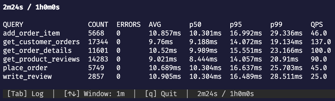
Queries display columns for count, errors, average latency, p90/p95/p99 latencies, and current QPS.

Transactions display columns for commits, rollbacks, errors, average latency, p90/p95/p99 latencies, and current TPS.

Chart view#

Shows a live time-series chart with one line per query or transaction:

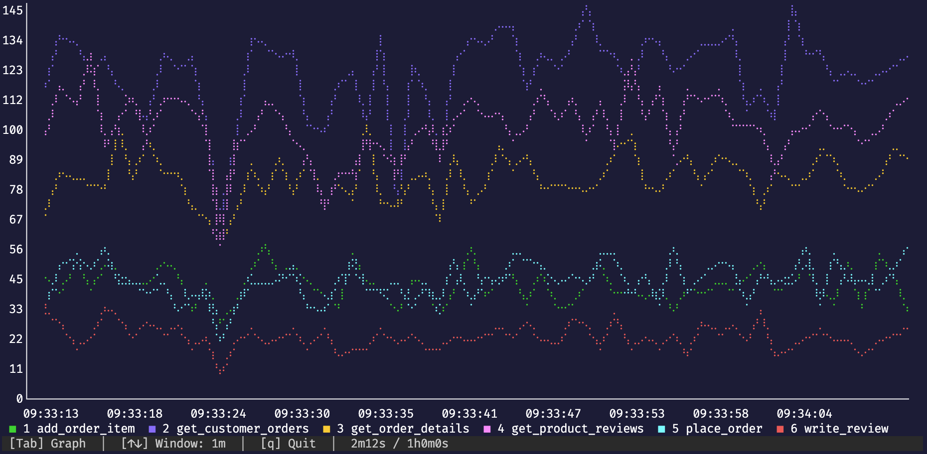
Each series is colour-coded and numbered in the legend at the bottom of the chart.

The chart defaults to QPS but you can cycle through five metrics using the ← / → arrow keys:

• QPS (queries/transactions per second)
• p90 latency (ms)
• p95 latency (ms)
• p99 latency (ms)
• Errors/s

The active metric is shown in the status bar at the bottom of the screen. Time window, series focus, and all other controls work the same regardless of which metric is selected.

Chart downsampling#

A run samples every --print-interval (default 1s), so a wide time window holds far more points than the chart has pixel columns - an hour of samples is roughly 3600 points across ~400 columns. Rather than plot them all and paint each column solid, the chart buckets points into one bucket per pixel column and plots a single value per bucket.

How a bucket collapses depends on the metric:

Narrowing the time window with ↑ / ↓ shrinks each bucket and brings back detail; at 1m each sample usually gets a column to itself and nothing is aggregated.

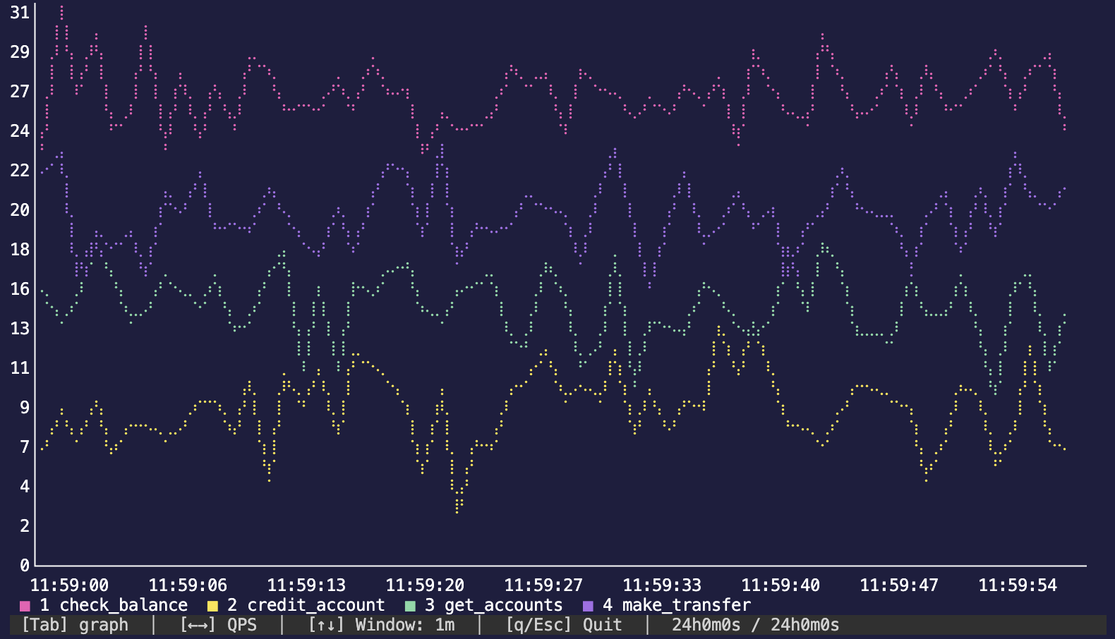
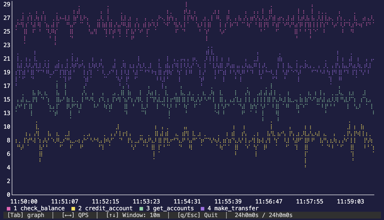
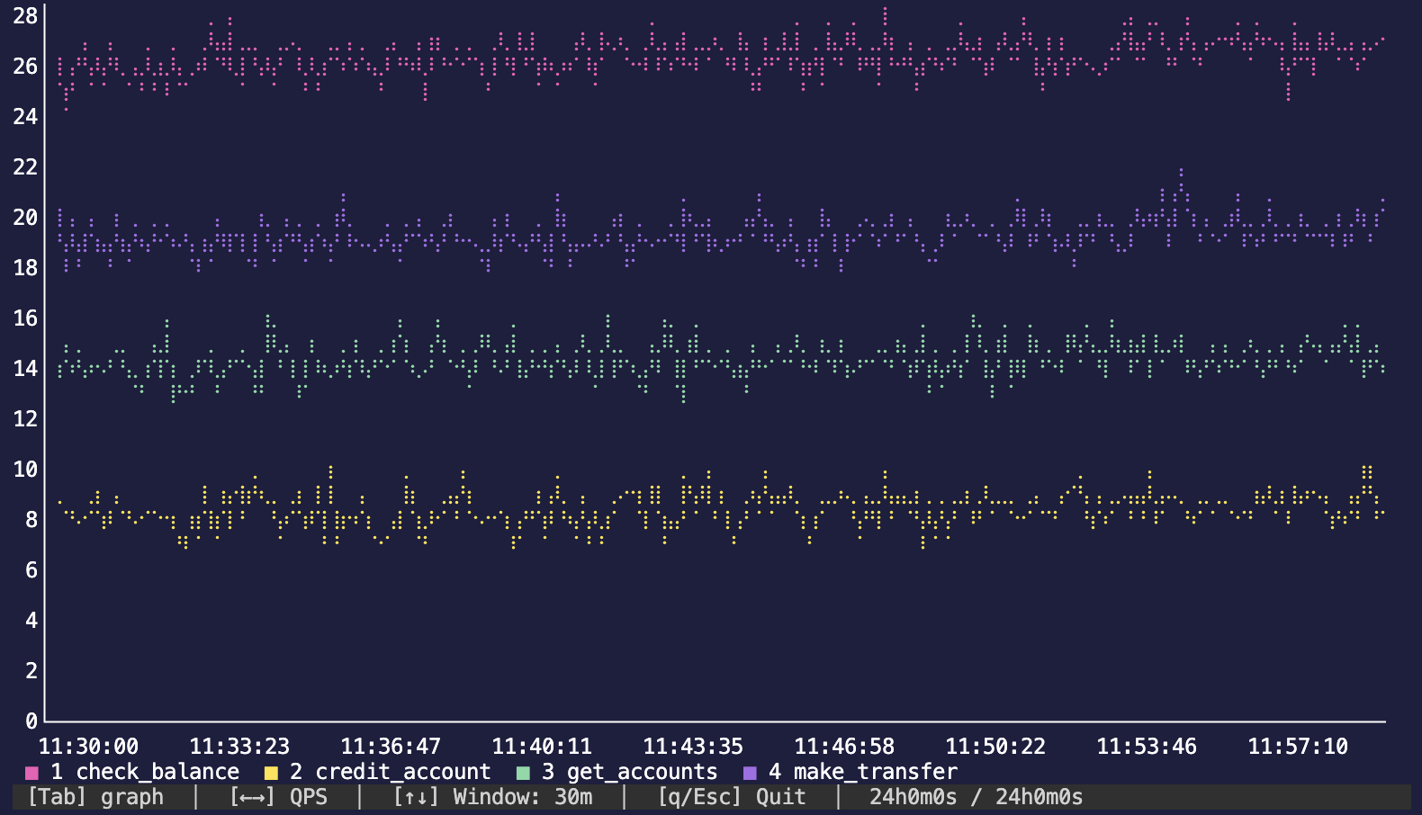
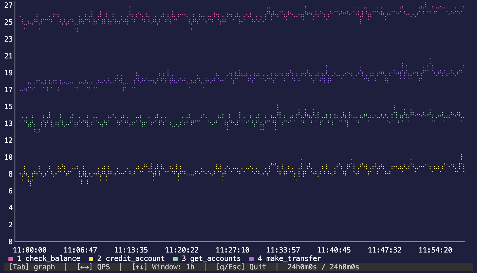
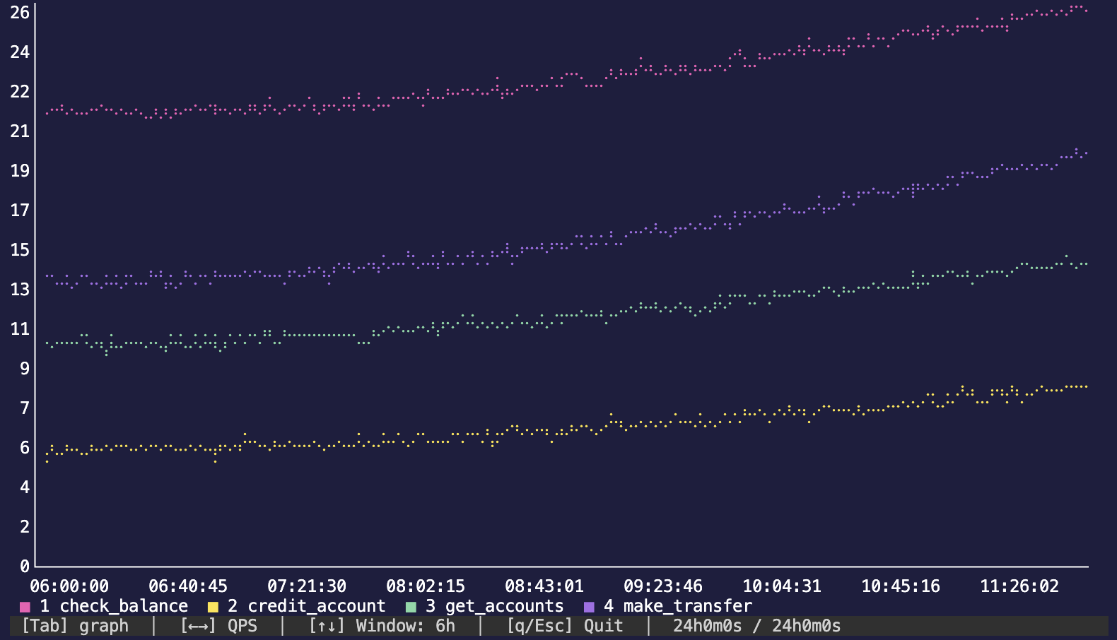
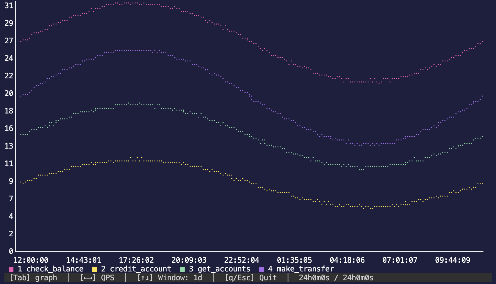
The same 24 hour run, seen through each window with ↑ / ↓. Widening trades per-sample detail for shape - the noise averages away and the daily cycle emerges:

1 Minute Window#

Every sample gets its own column, so nothing is aggregated and you see the raw per-tick jitter.

10 Minute Window#

A couple of samples per column. Still dominated by noise, but the band each series occupies is now obvious.

30 Minute Window#

A handful of samples per bucket. Still a noise band rather than a line, but each series sits clearly in its own lane.

1 Hour Window#

Roughly an order of magnitude more samples than columns. The band narrows and a slow upward drift becomes readable underneath it.

6 Hour Window#

Noise is essentially gone. Each series is a clean line.

1 Day Window#

The whole run in one frame, with the daily peak and overnight trough clearly separated.

Stats charts#

When a stats block uses post_print, the TUI Stats view renders an inline chart below the table. The chart type defaults to line but can be set to bar or gauge with the type node option.

The table lists every stats query’s values at once, but by default the chart shows one query at a time. Page between them with ←/→; the status bar names the current page and counts them, e.g. [←→] node (1/2). A query whose values appear in the table but not in the chart is a page away, not missing. Set layout on the block to put its queries on one page instead.

Block layout#

A stats block’s layout option controls how its queries share the Stats view:

stats (rate: 1 / 5s, layout: split) {
  node (
    type:       gauge,
    post_print: { key: 'under',       value: result().under },
    post_print: { key: 'unavailable', value: result().unavailable }
  ) `SELECT
       sum(under_replicated_ranges)::INT8 AS under,
       sum(unavailable_ranges)::INT8 AS unavailable
     FROM system.replication_stats`

  voters (
    type:       gauge,
    post_print: { key: 'min_live_voters', value: result().min_live_voters }
  ) `SELECT min(live_voters) AS min_live_voters FROM ranges`
}

Reach for merge when the queries are directly comparable and you want them on one scale, and split when they aren’t - a metric orders of magnitude larger than its neighbours will flatten them on a shared axis, but not in its own pane.

layout applies within a block. Separate blocks remain separate pages, so a run with two merged blocks still pages between them. To get everything onto one page, put the queries in one block.

Two things to know:

• merge requires one chart type. Merging draws the queries into a single chart, which can only be one shape, so a block mixing bar and line is a config error. Labels are prefixed with the query name (node/under) so two queries using the same print key stay apart.
• split falls back to paging when it can’t fit. Below about 24 columns per chart the block pages as if layout: page, and goes back to splitting when the terminal is widened. Focus keys (1-9) select nothing on a split page, since each chart has its own series.

Line chart (default)#

A line chart plots a numeric value over time. It is the default when no type is specified:

stats (rate: 1 / 1s) {
  latency (
    post_print: { key: 'p99', value: result().p99_ms }
  ) `SELECT p99_ms FROM latency_stats`
}

Bar chart#

A bar chart shows the frequency distribution of a categorical value. Set type: bar on the node:

stats (rate: 1 / 1s) {
  node (type: bar) (
    post_print: { key: 'id', value: result().node_id }
  ) `SHOW node_id`
}

Gauge chart#

A gauge chart draws one bar per print expression, with the bar’s height set to that expression’s latest value. Where a bar chart counts how often each distinct value was seen, a gauge tracks the value itself, so the bars rise and fall with the metric. Set type: gauge on the node:

stats (rate: 1 / 5s) {
  ranges (
    type:       gauge,
    post_print: { key: 'under',       value: result().under },
    post_print: { key: 'unavailable', value: result().unavailable }
  ) `
    SELECT
      sum(under_replicated_ranges)::INT8 AS under,
      sum(unavailable_ranges)::INT8 AS unavailable
    FROM system.replication_stats`
}

This is the shape you want for current-state numbers you’d otherwise read off a dashboard - replica counts, queue depths, connection counts - where the comparison between metrics matters more than their history. Reach for a line chart instead when you care how a value got where it is.

All the bars share one y-axis, so metrics with wildly different magnitudes flatten each other. Split those across separate stats nodes.

Each bar shows the mean over the last print interval that produced a sample, so a query polled slower than --print-interval holds its last value rather than dropping to zero. Add window to a print expression to average over a longer span and steady a noisy bar.

Bar labels carry the current value (under 0), so a gauge whose metrics are all zero still reads as zero rather than as a chart that failed to draw.

One line per distinct value#

A bar chart shows you what the distribution is right now, but not how it got there. Set series: value on a line chart’s print expression to plot one coloured line per distinct value the expression returns, with the y-axis showing how many times per second that value was seen:

stats (rate: 20 / 1s) {
  node (type: line) (
    post_print: { key: 'node', value: result().node_id, series: value, window: 5s }
  ) `SHOW node_id`
}

This is the shape you want for rolling upgrades, node drains, and rebalancing - anywhere the interesting signal is how a mix shifts over time. Poll fast (e.g. rate: 20 / 1s) so each line has enough samples to be smooth.

Series are named from the values themselves and keep their colour for the whole run. A value that stops appearing drops to zero rather than vanishing from the chart, so you can see a node leave the cluster or an old version drain away.

Values are treated as categorical even when they’re numeric, so the stats table shows a frequency breakdown (1=412 2=398 3=405) rather than min/avg/max. If more than one print expression on the same node uses series: value, the lines are prefixed with their key to make them easier to tell apart.

Aggregation window#

By default an aggregation covers the whole run, so a long run’s numbers converge and stop reacting to what’s happening now. Set window to a duration to aggregate over a sliding window instead:

stats (rate: 1 / 1s) {
  latency (
    post_print: { key: 'p99', value: result().p99_ms, window: 30s }
  ) `SELECT p99_ms FROM latency_stats`
}

The window is rounded to the nearest multiple of --print-interval (default 1s) and covers at least one interval, so window: 500ms behaves the same as window: 1s. Values older than the window age out of the table, the bar chart, and the series: value rates.

How the three rates interact#

A windowed stats query has three separate numbers, and it’s easy to assume they’re related when they aren’t:

stats (rate: 1 / 1s) {                                    # block rate
  version_over_time(
    type:       line,
    rate:       20 / 1s,                                  # query rate
    post_print: {
      key: 'version',
      value: result().version,
      series: value,
      window: 10s                                         # sliding window size
    }
  ) `SELECT split_part(version(), ' ', 3) AS version`
}

The window is divided into buckets of one --print-interval each (not one block tick each). With the default --print-interval of 1s, a window: 10s is a ring of 10 buckets, each holding one second of observations. At rate: 20 / 1s that’s ~20 samples per bucket and ~200 across the window.

The consequences:

• Changing --print-interval changes the resolution, not the span. At --print-interval 2s, a window: 10s becomes 5 buckets - still 10 seconds, but a change in the data snaps in 2-second steps.
• Changing the query rate changes samples per bucket only. It makes the line smoother or noisier; it does not make the window longer or shorter.
• Changing window changes how long a value lingers after it stops appearing.

Counts in the stats table read slightly below rate * window, because the newest bucket is still filling when the table is rendered. At 20/s over a 10s window, expect roughly 180–200 rather than exactly 200.

Series that stop appearing#

The chart and the stats table treat a value that drops out of the window differently:

• The chart knows every value seen for the lifetime of the run and plots a missing one as zero, so a node leaving the cluster or an old version draining away falls to the axis instead of vanishing.
• The stats table only lists values actually seen inside the window. Once a value ages out completely, its key=count entry disappears from the row.

So during a rolling upgrade with window: 10s, the table shows both versions only for the ~10 seconds they overlap in the window:

version_over_time  version  v25.3.1=54 v26.2.4=138     # mid-switch
version_over_time  version  v26.2.4=196                # 10s later

Widen the window if you want the old value to stay visible in the table for longer. Frequency rows list at most 10 values, sorted by value.

Keyboard shortcuts#

The chart key wraps to as many lines as the terminal width needs, and the chart gives up the rows it takes, so a run with a lot of series still fits on screen.

Pausing before teardown#

With --pause, edg all holds the TUI on screen once the run finishes instead of exiting into a plain prompt, so the final chart stays readable while you query the database. The clock freezes with it - the time window stops sliding, so the data cannot scroll out from under you. The status bar swaps [q/Esc] Quit for [Enter/q] Deseed and down; either key resumes, and teardown runs as usual afterwards.